Results — causal importance

Archive — the original J-space replication study

This is what the repository started as: replicating the J-space / global-workspace readout claim on open weights. That readout claim did not survive our controls — an informative null, preserved here with full rigor — and the project pivoted to the operator/operand finding on the main page. These pages are kept as-is.

Is the J-space merely readable, or does it actually steer the computation? Using the paper's shipped two-hop probe-swap set, we move the residual component along a bridge entity's J-lens direction onto a different entity's direction, across a layer band, and check whether the model's greedy answer flips accordingly — against a matched-norm random control.

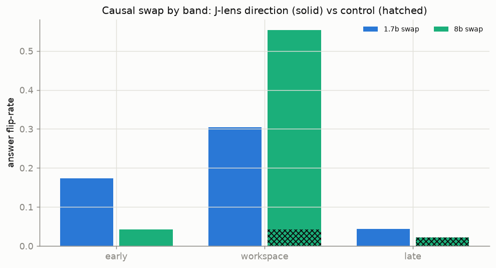
The workspace band is causally potent — and sharpens with scale

model	early	workspace	late	control	n solved
1.7B	0.17	0.30	0.04	0.00	23
8B	0.04	0.55	0.02	0.04	47

This is the project's cleanest result. Three things:

1. The workspace band dominates, at both scales — exactly where the paper locates the workspace.
2. The control does nothing. A random direction of identical norm never produces the swapped answer, so the effect is specific to the J-lens directions, not to perturbation magnitude.
3. It sharpens with scale. From 1.7B to 8B the workspace flip-rate nearly doubles (0.30 → 0.55) and localizes: the early band collapses (0.17 → 0.04), so at 8B the workspace is ~14× more causally potent than the early/late bands (vs ~2× at 1.7B). The global workspace becomes both stronger and more sharply localized as the model grows.

The striking dissociation: this causal structure is strong before any readout advantage appears (see scale) — the workspace steers the two-hop even though the J-lens does not yet out-read the logit-lens on Qwen3.

In progress

32B (int8) is the third point; the question is whether the workspace sharpening continues.

Channels: workspace → output

A complementary view of how a concept reaches the output. For a two-hop probe we project the residual — transported into the final basis by the J-lens — onto a 2D plane spanned by two concept tokens (the intermediate and the answer), and trace the path layer by layer.

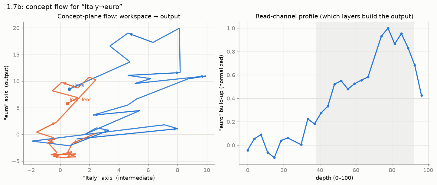
• Right — read-channel profile. The build-up of the answer concept along depth: it climbs steeply through the workspace band and peaks late — this is literally which layers assemble the output.
• Left — concept-plane flow. The J-lens path (blue) travels far across the concept plane, while the logit-lens path (orange) stays cramped near the origin — a visual of why the untransported logit lens under-reads the middle of the network (see Method).

Metaphor, and a small model

Attention mixes positions, so this is a projected trajectory, not an autonomous vector field — "streamline" is a visual metaphor for the path. At 1.7B the J-lens path is jagged (an immature workspace); the 8B/32B versions should be smoother and move more cleanly from the intermediate axis to the output axis.